From Perceptron to Deep Neural Nets
As a machine learning engineer, I have been learning and playing with deep learning for quite some time. Now, after finishing all Andrew NG newest deep learning courses in Coursera, I decided to put some of my understanding of this field into a blog post. I found writing things down is an efficient way in subduing a topic. In addition, I hope that this post might be useful to those who want to get started into Deep Learning.
Alright, so let us talk about deep learning. Oh, wait, before I jump directly
talking about what a Deep Learning or a Deep Neural Network (DNN) is, I would
like to start this post by introducing a simple problem where I hope it will
give us a better intuition on why we need a (deep) neural network. By the way, together with this post I am also releasing code on
Github
that allows you to train a deep neural net model to solve the XOR problem below.
XOR PROBLEM
The XOR, or “exclusive or”, problem is a problem where given two binary inputs,
we have to predict the outputs of a XOR logic gates. As a reminder, a XOR
function should return 1 if the two inputs are not equal and 0 otherwise. Table
1 below shows all the possible inputs and outputs for the XOR function:
| X1 | X2 | Output |
|---|---|---|
| 1 | 1 | 0 |
| 1 | 0 | 1 |
| 0 | 1 | 1 |
| 0 | 0 | 0 |
Now, let us plot our dataset and see how is the nature of our data.
def plot_data(data, labels):
    """
    argument:
    data: np.array containing the input value
    labels: 1d numpy array containing the expected label
    """

    positives = data[labels == 1, :]
    negatives = data[labels == 0, :]
    plt.scatter(positives[:, 0], positives[:, 1],
                        color='red', marker='+', s=200)
    plt.scatter(negatives[:, 0], negatives[:, 1],
                        color='blue', marker='_', s=200)

    positives = np.array([[1, 0], [0, 1]])
    negatives = np.array([[0, 0], [1, 1]])
    data = np.concatenate([positives, negatives])
    labels = np.array([1, 1, 0, 0])

    plot_data(data, labels)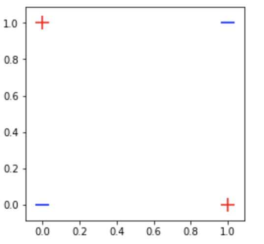
Maybe after seeing the figure above, we might want to rethink whether this xor problem is indeed a simple problem or not. As you can see, our data is not linearly separable, hence, some well-known linear model out there, such as logistic regression might not be able to classify our data. To give you a clearer understanding, below I plot some decision boundaries that I built using a very simple linear model:
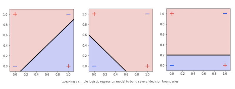
Having seen the figure above, it is clear that we need a classifier that works well for non-linearly separable data. SVM with its kernel trick can be a good option. However, in this post, we are going to build a neural network instead and see how this neural network can help us to solve the XOR problem.
What is Neural Network?
Neural Network or Artificial Neural Network is a very good function approximators that based loosely on the ways in which the brain is believed to work. Figure 1 below shows the analogy between the human biological neuron and an artificial neural network.

Figure 1. (a) Structure of neurons in brain (b) Analogy of Artificial Neural Network With Biological Neural Network — image taken from cs231n.github.io
Without going into too much detail on a biological neuron, I will give a
high-level intuition on how the biological neuron process an information.
Our neuron receives signals through Dendrite. This information or signals are then passed through to the Soma or the Cell Body. Inside the cell body, all of the information will be summed up to generate an output. When the sumed up result reaches a threshold value, the neuron fires and the information will be carried down through the axon, then to other connected neurons through its synapses. The amount of signal transmitted between neurons depends upon the strength of the connections.
The whole aforementioned flow is something that is adopted by the artificial neural network. You can think of the dendrite as the weighted inputs based on their synaptic interconnection in an artificial neural network. The weighted input is then summed up together inside a ‘cell-body’ of the artificial neural network. If the generated output is greater than the threshold unit, the neuron will “fire” and the output of this neuron will be transferred to the other neurons.
So, you can see that the ANN is modeled using the working of basic biological neurons.
So, How do this Neural Network works?
In order to know how this neural network works, let us first see a very simple form of an artificial neural network called Perceptron.
For me, Perceptron is one of the most elegant algorithms that ever exist in machine learning. Created back in the 1950s, this simple algorithm can be said as the foundation for the starting point to so many important developments in machine learning algorithms, such as logistic regression, support vector machine and even deep neural networks.
So how does a perceptron works? We’ll use a picture represented in Figure 2 as the starting point of our discussion.
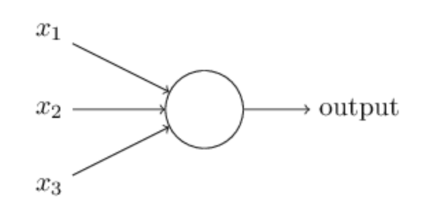
Figure 2. Perceptron — Source
Figure 2 shows a perceptron algorithm with three inputs, x1, x2 and x3 and a neuron unit which can generate an output value. For generating the output, Rosenblatt introduced a simple rule by introducing the concept of weights. Weights are basically real numbers expressing the importance of the respective inputs to the output [1]. The neuron depicted above will generate two possible values, 0 or 1, and it is determined by whether the weighted sum of each input, ∑wjxj, is less than or greater than some threshold value. Therefore, the main idea of a perceptron algorithm is to learn the values of the weights w that are then multiplied with the input features in order to make a decision whether a neuron fires or not. We can write this in a mathematical expression as depicted below:

Now, we can modify the formula above by doing two things: First, we can transformed the weighted sum formulation into a dot product of two vectors, w (weights) and x (inputs), where w⋅x ≡ ∑wjxj. Then, we can move the threshold to the other side of the inequality and to replace it by a new variable, called bias b, where b ≡ −threshold. Now, with those modification, our perceptron rule can be rewritten as:

Now, when we put all together back to our perceptron architecture, we’ll have a complete architecture for a single perceptron as depicted below:
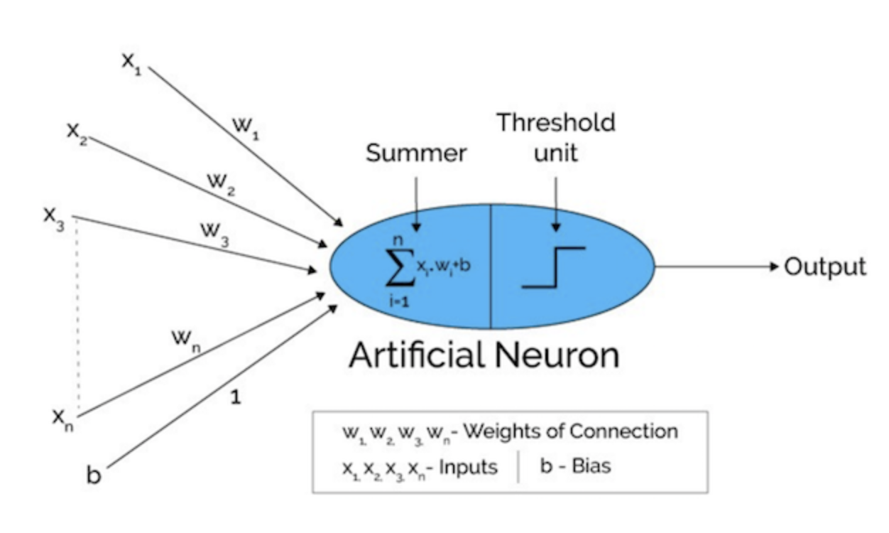
Figure 3. A single layer perceptron architecture
A typical single layer perceptron uses the Heaviside step function as the activation function to convert the resulting value to either 0 or 1, thus classifying the input values as 0 or 1. As depicted in Figure 4, the Heaviside step function will output zero for negative argument and one for positive argument.
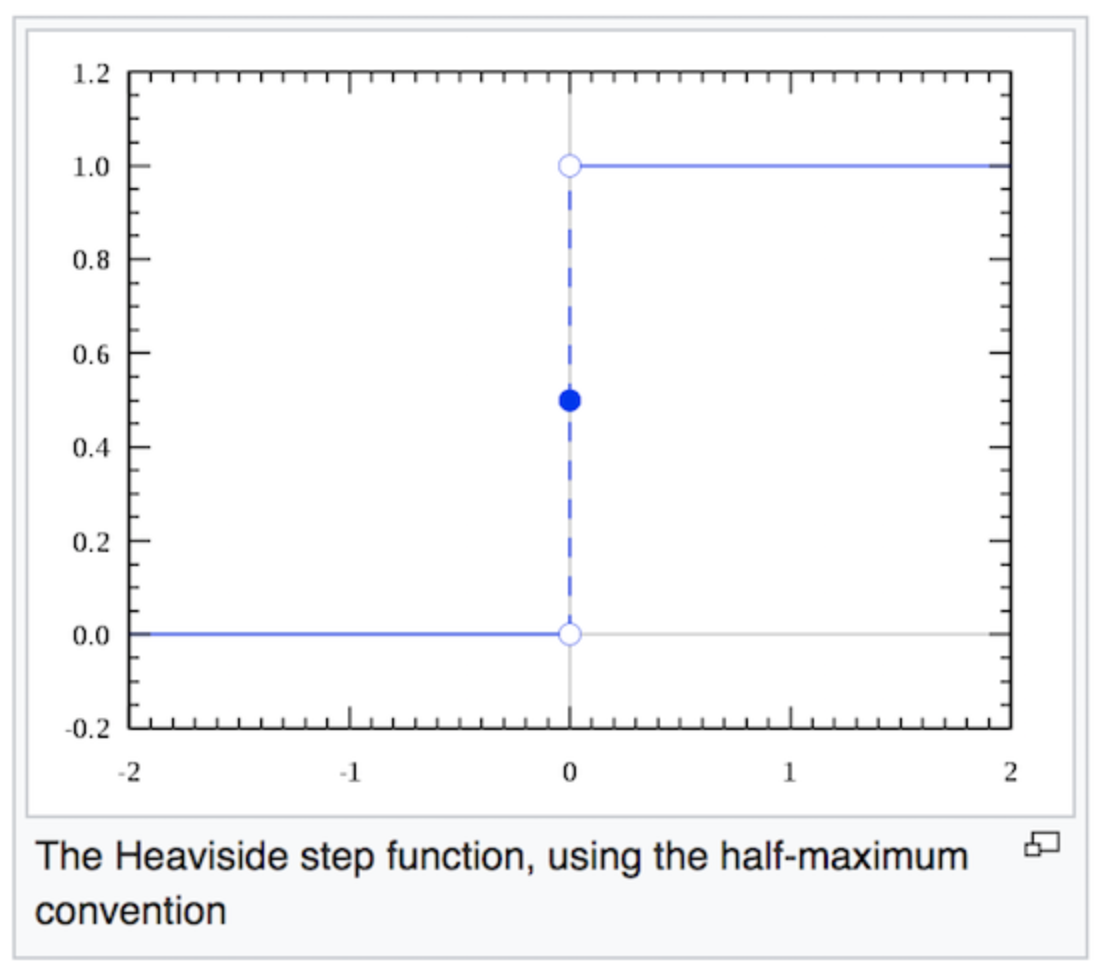
Figure 4. The shape of the Heaviside step function — Source
The Heaviside step function is particularly useful in classification task in cases where the input data is linearly separable. However, recall that our goal is to find a classifier that works well in a non linearly separable data. Therefore, both a single layer perceptron and the Heaviside step function is obviously pointless here. Later, as you’ll see in the next section, we’ll need to have a multiple layers that consists of several perceptrons along with a non linear activation function.
Specifically, there are two main reasons why we cannot use the Heaviside step function —( see also my answer on stats.stackexchange.com):
-
At the moment, one of the most efficient ways to train a multi-layer neural network is by using gradient descent with backpropagation (we’ll talk about these two methods shortly). A requirement for backpropagation algorithm is a differentiable activation function. However, the Heaviside step function is non-differentiable at x = 0 and it has 0 derivative elsewhere. This means that gradient descent won’t be able to make a progress in updating the weights.
-
Recall that the main objective of the neural network is to learn the values of the weights and biases so that the model could produce a prediction as close as possible to the real value. In order to do this, as in many optimisation problems, we’d like a small change in the weight or bias to cause only a small corresponding change in the output from the network. Having a function that can only generate either 0 or 1 (or yes and no), won’t help us to achieve this objective.
Activation Function
The activation function is one of the most important components in the neural network. In particular, a nonlinear activation function is essential at least for three reasons:
- It helps the neuron to learn and make sense of something really complicated.
- They introduce nonlinear properties to our Network.
- we’d like a small change in weight to cause only a small corresponding change in the output from the network
We’ve seen that the Heaviside step function as one example of an activation function, nevertheless, in this particular section, we’ll explore several non-linear activation functions that are generally used in the deep learning community. By the way, a more in-depth explanation of the activation function, including the pros and cons of each non-linear activation function, can be studied in these two great post written by Avinash Sharma and Karpathy.
Sigmoid Function
The sigmoid function, also known as the logistic function, is a function that given an input, it will generate an output in range (0,1). The sigmoid function is written as:
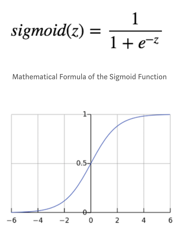
Figure 5. The shape of the Sigmoid Function
Figure 5 draws the shape of the sigmoid function. As you can see, it is like the smoothed out version of the Heaviside step function. However, the sigmoid function is preferable due to many factors, such as:
- It is nonlinear in nature.
- Instead of outputing 0 and 1, now we have a function that can give a value output 0.67. Yup, as you might guess, this can be used to represent a probability value.
- Still related to point (2), now we have our activations bound in a range, which means it won’t blow up the activations.
However, the sigmoid activation function has some drawbacks:
The vanishing gradient. As you can see from the preceding figure, when z, the input value to the function, is really small (moving towards -inf), the output of the sigmoid function will be closer to zero. Conversely, when z, is really big (moving towards +inf), the output of the sigmoid function will be closer to
So what does this imply?
In that region, the gradient is going to be very small and even vanished. The vanishing gradient is a big problem especially in deep learning, where we stack multiple layers of such non-linearities on top of each other, since even a large change in the parameters of the first layer doesn’t change the output much. In other words, the network refuses to learn and oftentimes the time taken to train the model tend to become slower and slower, especially if we use the gradient descent algorithm.
Another disadvantage of the sigmoid activation function is that computing the exponential can be expensive in practice. Although, arguably, the activation function is a very small part of the computation in a deep net compared to the matrix multiplication and/or convolution, so, this might not become a huge problem. However, I think it is worth to mention.
Tanh Function
Tanh or hyperbolic tangent is another activation function that is commonly used in deep neural nets. The nature of the function is very similar to the sigmoid function where it squash the input into a nice bounded range value. Specifically, given a value, tanh will generate an output value between -1 and 1.
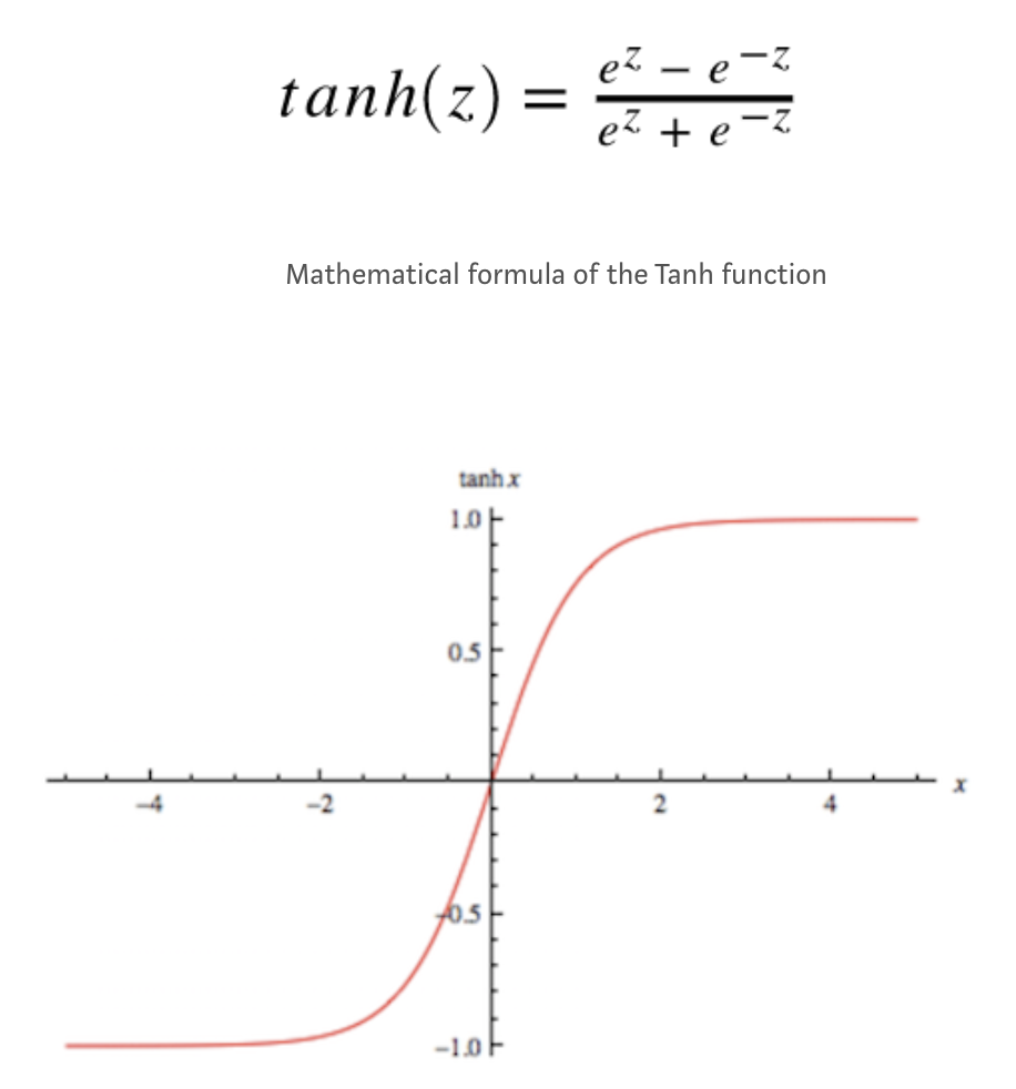
Figure 6. The shape of the tanh function
As mentioned earlier, the tanh activation function has characteristics similar to the sigmoid function. It is nonlinear and it is bound to a certain range, in this case (-1, 1). Also, not surprisingly, tanh shares the same drawbacks as what the sigmoid has. It suffers from the vanishing gradient problem and as you can see from the mathematical formula, we need to compute the exponential, which oftentimes is computationally inefficient.
ReLu (Rectified Linear Unit)
Here it comes the ReLu, an activation function that was not expected to perform better than sigmoid and tanh, yet, in practice it does! In fact, this lecture says by default, use the ReLU non-linearity.
The ReLu has a very nice mathematical property in which it is very computationally efficient. Given an input value, the ReLu will generate 0, if the input is less than 0, otherwise the output will be the same as the input. Mathematically speaking, this is the form of the ReLu function
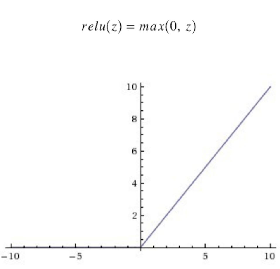
Figure 7. The shape of the ReLu function
Now, you may ask, “isn’t that a linear function? why do we call ReLu as a nonlinear function?”
First, let us first understand what a linear function is. Wikipedia says that:
In linear algebra, a linear function is a map f between two vector spaces that preserves vector addition and scalar multiplication:
f(x + y) = f(x) + f(y)
f(ax) = af(x)
Given the definition above, we can see that max(0, x) is a piece-wise linear function. It is piece-wise because it is linear only if we restrict its domain to (−inf, 0] or [0,+inf). However, it is not linear over its entire domain. For instance
f(−1) + f(1) ≠f (0)
So, now we know that ReLu is a nonlinear activation function and it has a nice mathematical property and also computationally more efficient compared to sigmoid or Tanh. In addition, ReLu is known to be “free” from the vanishing gradient problem. However, there is one big drawback in ReLu, which is called the “dying ReLu”. The dying ReLu is a phenomenon where a neuron in the network is permanently dead due to inability to fire in the forward pass.
To be more precise, this problem occurs when the activation value generates by a neuron is zero while in forward pass, which resulting that its weights will get zero gradient. As a result, when we do backpropagation, the weights of that neuron will never be updated and that particular neuron will never be activated. I highly suggest you to watch this lecture video which has more in-depth explanation on this particular problem and how to avoid the dying ReLu problem. Please go check it!
Oh, one more thing about ReLu that I think worth to mention. As you may notice, unlike the sigmoid and tanh, ReLu doesn’t bound the output value. As this might not become a huge problem in general, it can be, however, become troublesome in another variant of deep learning model such as the Recurrent Neural Network (RNN). Concretely, the unbounded value generated by the ReLu could make the computation within the RNN likely to blow up to infinity without reasonable weights. As a result, the learning can be remarkably unstable because a slight shift in the weights in the wrong direction during backpropagation can blow up the activations during the forward pass. I’ll try to cover more about this in my next blog post, hopefully :)
How does a Neural Network Predicts and Learns?
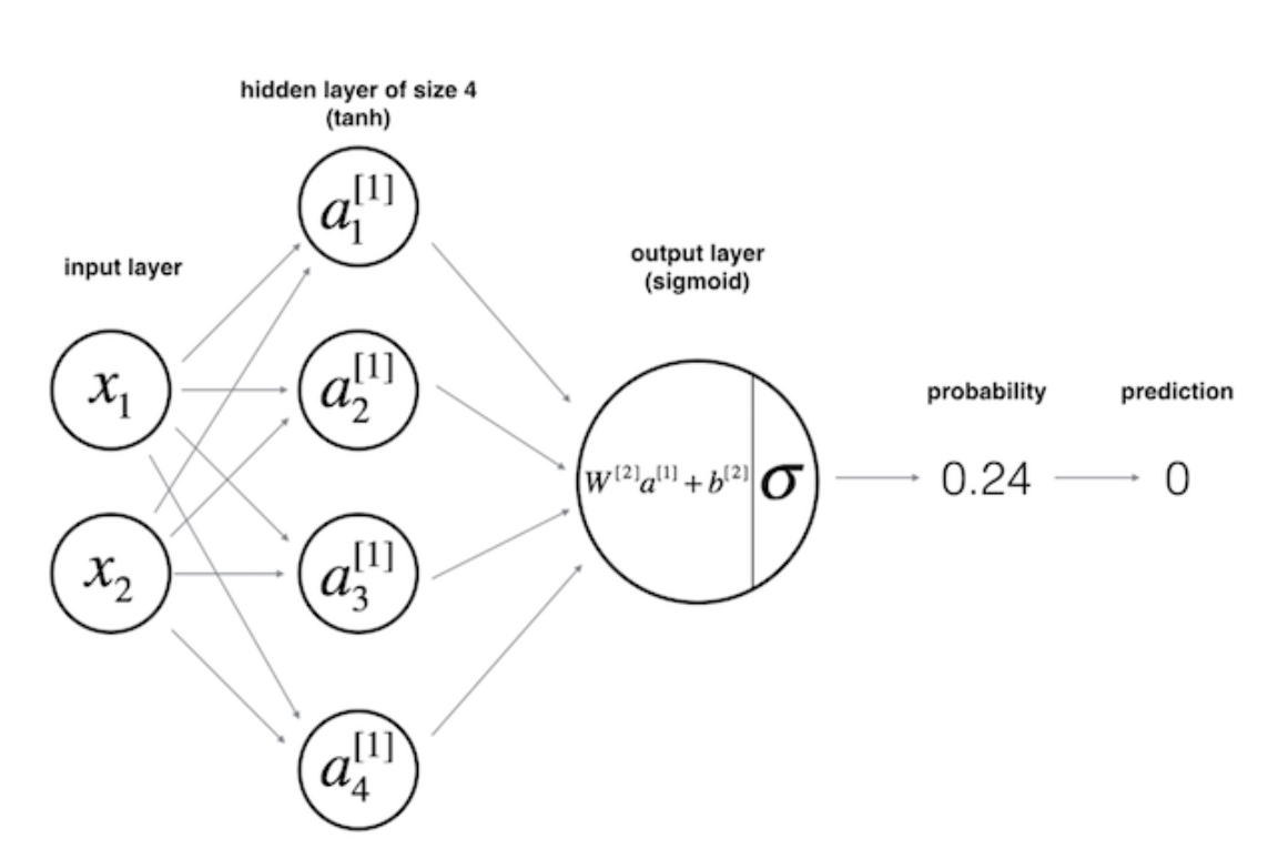
Figure 8. The Multi Layer Perceptrons
The architecture depicted in Figure 8 above is called the multi-layer perceptrons (MLP). As its name implies, in MLP, we simply stacked multiple perceptrons into several layers. The one depicted above is a network with 3 layers: an input layer, a hidden layer, and an output layer. However, in the deep learning or neural net community, people don’t call this network as three layers neural network. Usually, we just count the number of hidden layers or number of hidden layer along with the output layer, hence two-layers neural network. The hidden layers simply mean neither an input nor an output layer. Now, as you might guess, the term deep learning solely implies, we have “more” hidden layers :).
So how do a neural net generates a predictions?
A neural network generates a prediction after passing all the inputs through all the layers, up to the output layer. This process is called feedforward. As you can see from Figure 8, we “feed” the network with the input, x, compute the activation function and pass it through layer by layer until it reaches the output layer. In supervised setting task, such as classification task, we usually use a sigmoid activation function in the output layer since we can translate its output as a probability. In Figure 8, we can see that the value generated by the output layer is 0.24, and since this value is less than 0.5, we can then said the prediction, y_hat, is zero.
Then, as in typical classification task, we’ll have a cost function which measures how good our model approximate the real label is. In fact, training in neural network simply means, minimize the cost as much as possible. We can define our cost function as follows:

Mean Squared Error
So the objective is to find some combination of w’s and b that could make our cost J, as small as possible. To do this, we’ll rely on two important algorithms which are Gradient Descent and Backpropagation.
Gradient Descent Algorithm
For those of you who have been doing machine learning might already know about the gradient descent algorithm. Training a neural network is not much different from training any other machine learning model with gradient descent. The only notable difference would be the effect of nonlinearities in our network that makes our cost function become non-convex.
To give a better intuition, let us assume that our cost function is a convex function (a big one bowl) as depicted in Figure 9 below:
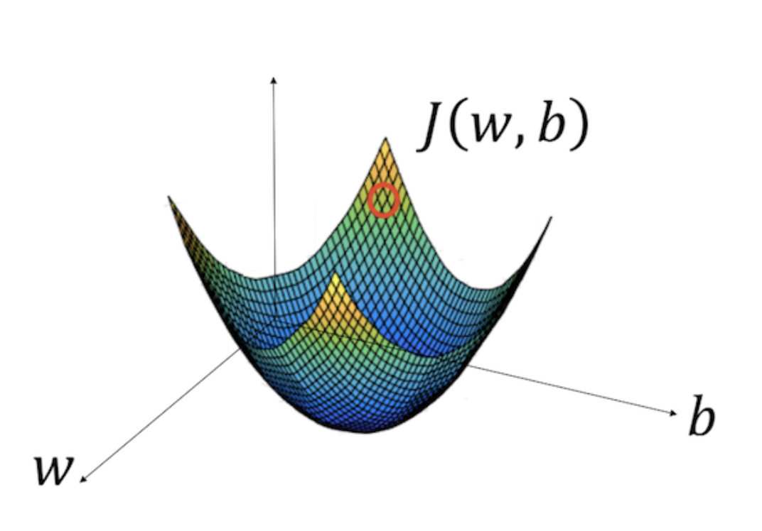
Figure 9. The schematic of the Gradient Descent — Source
In the diagram above, the horizontal axes represent our space of parameters, weights and biases, while the cost function, J(w, b) is then some surface above the horizontal axes. The red circle depicted in the diagram above is the original value of our cost w.r.t the weights and bias. To minimize the cost, we now know that we have to go to the steepest path down the bowl. But the question is, how do we know which direction to step? Should we increase or decrease the value of our parameters? We can do a random search, but it will take quite a long time and obviously computationally expensive.
There is a better way to find which direction we should go, in tweaking the learnable parameters, weights and biases. Calculus teaches us that the direction of the gradient vector, at a given point, will naturally point in the steepest direction. Therefore, we’ll use the gradient of our cost function w.r.t our weights and our biases.
Now, Let us simplify things by just looking the cost w.r.t the weights as depicted in Figure 10 below:
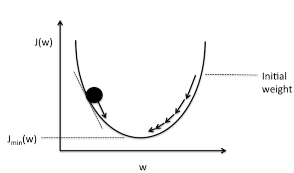

Figure 10. Visualization of negative and positive gradients — source
Figure 10 pictures the value of our cost function w.r.t to the value of the weights. You can think of the black circle above as our original cost. Recall that the gradient of a function or a variable can be positive, zero or negative. A negative gradient means that the line slopes downwards and vice versa if it is positive. Now, since our objective is to minimize the cost, we then need to move our weights in the opposite direction of the gradient of the cost function. This update procedure can be written as follow:
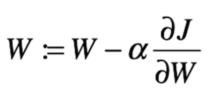
Figure 11. Parameters update — Gradient Descent
where α is a step size or learning rate and we’ll multiply this with the partial derivative of our cost w.r.t the learnable parameters. So, what does α used for?
Well, the gradient tells us the direction in which the function has the steepest rate, however, it does not tell us how far along this direction we should step. Here is where we need the α, which is a hyperparameter that basically control the size of our step, like, how much should we move towards a certain direction. Choosing the right value for our learning rate is very important since it will hugely affect two things: the speed of the learning algorithm and whether we can find the local optimum or not (converge). In practice, you might want to use an adaptive learning rate algorithms such as momentum, RMSProp, Adam and so forth. A guy from AYLIEN wrote a very nice post regarding various optimization and adaptive learning rate algorithm.
Backpropagation
In the previous section, we’ve talked about the gradient descent algorithm, which is an optimization algorithm that we use as the learning algorithm in a deep neural network. Recall that by using gradient descent means that we need to find the gradient of our cost function w.r.t our learnable parameters, w, and b. In other words, we need to compute the partial derivative of our cost function w.r.t w and b.
However, if we observe our cost function J, as depicted in Figure 12 below, there is no a direct relationship between J and both w and b.

Figure 12. Mean Squared Error
Only if we trace back from the output layer, the layer that generates y_hat, way to the input layer, we’ll see that J has an indirect relation with both w and b, as shown in Figure 13 below:
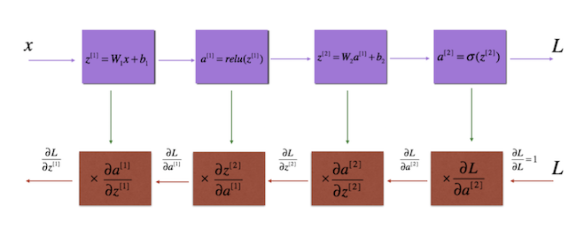
Figure 13. The schematic of the backpropagation
Now, you can see that in order to find the gradient of our cost w.r.t both w and b, we need to find the partial derivative of the cost with all the variables, such as a (the activation function) and z (the linear computation: wx + b) in the preceding layers. This is where we need a backpropagation. Backpropagation is basically a repeated application of chain rule of calculus for partial derivatives, which I would say, probably the most efficient way to find the gradient of our cost J w.r.t to all the learnable parameters in a neural network.
In this post, I’ll walk you to compute a gradient of the cost function J w.r.t W2, which is the weights in the second layer of a neural network. For simplicity, we’ll use the architecture shown in Figure 8, where we have one hidden layer with three hidden neurons.
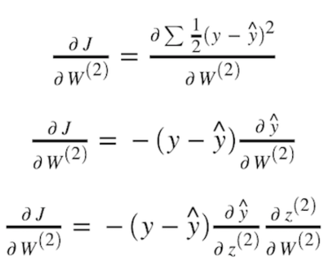
To find the rate of change of y_hat w.r.t z2, we need to differentiate our sigmoid activation function with respect to z. Assuming we use a sigmoid activation function, we can then compute it as:
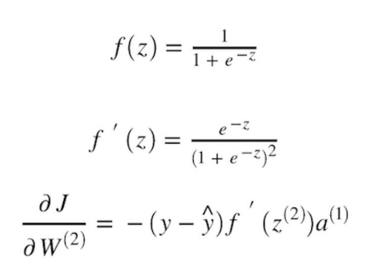
Now, once we have the value of our partial derivative J w.r.t W2, we can update the value of our W2 using the formula shown in Figure 11 in the previous section. Basically, we’ll perform the same computation with all the weights and biases repeatedly until we have a cost value as minimum as possible.
Neural Nets for Solving the XOR Problem
Great! I guess we’ve covered pretty much everything that we need to know in order to build a neural network model, and even a deep learning model, that would help us to solve the XOR problem.
While writing this post, I’ve built a simple neural network model with only one hidden layers with various number of hidden neurons. The example of the network that I used is shown in Figure 14 below. Also, I presented some decision boundaries generated by my model with different number of neurons. As you can see later, we can say that having more neurons will make our model become more complex, hence creating a more complex decision boundary.
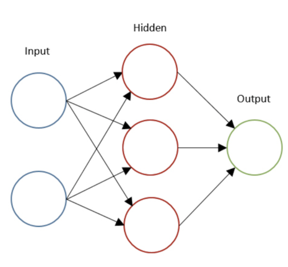
Figure 14. A two layers neural net with 3 hidden Neurons

Figure 15. Decision boundaries generated by one hidden layer with several hidden neurons
But, what would be the best choice? having more neurons or going deeper, meaning having more layers?
Well, Theoritically, the main benefit of a very deep network is that it can represent very complex functions. Specifically, by using a deeper architecture, we can learn features at many different levels of abstraction, for instance identifying edges (at the lower layers) to very complex features (at the deeper layers).
However, using a deeper network doesn’t always help in practice. The biggest problem that we will encounter when training a deeper network is the vanishing gradients problem: a condition where a very deep networks often have a gradient signal that goes to zero quickly, thus making gradient descent unbearably slow.
More specifically, during gradient descent, as we backprop from the final layer back to the first layer, we are multiplying by the weight matrix on each step, and thus the gradient can decrease exponentially quickly to zero or, in rare cases, grow exponentially quickly and “explode” to take very large values.
So, to wrap up this lengthy post, these are a few bullet points that would briefly summarise it:
- The intuition, the Neural Net introduces non-linearities to the model and can be used to solve a complex non-linearly separable data.
- Perceptron is an elegant algorithm that powered many of the most advancement algorithms in machine learning, including deep learning.
- Intuitively, deep learning means, use a neural net with more hidden layers. Of course, there are many variants of it, such as Convolution Neural Net, Recurrent Neural net and so on.
- Activation function is extremely an important component in neural net and YES, you should understand it.
- Currently, Gradient Descent with Backpropagation is the best combination that we use to train a (deep) Neural Net.
- Having more hidden layers not necessarily improves the performance of our model. In fact, it suffers from one well-known problem called the vanishing gradient problem.
Adi Chris
A passionate learner and the machine learning enthusiast.